---
title: "Integrals in Probability"
bibliography: "../../blog.bib"
author: "Peter Amerkhanian"
date: "2024-4-14"
draft: false
description: "Notes on the definite integral and probability modeling, with a mix of formal notation, `plotly` visuals, and `sympy` computation."
image: thumbnail.png
jupyter: python3
engine: knitr
categories: ['R', 'Calculus', 'Probability']
format:
html:
toc: true
toc-depth: 3
code-fold: false
code-tools: true
editor:
markdown:
wrap: 72
---
```{r}
#| warning: false
#| code-fold: true
library(plotly)
library(dplyr)

x_vec <- seq(0, 25)
y_vec <- seq(0, 25)

vline <- function(x = 0, color = "black") {
  list(
    type = "line",
    y0 = 0,
    y1 = 1,
    yref = "paper",
    x0 = x,
    x1 = x,
    line = list(color = color, dash="dot")
  )
}
```
The following are notes on using integration for finding cumulative probability distribution functions in the univariate and joint settings. The exercises and citations are all coming out of a textbook for a course in vector calculus [@strang_calculus_2016-1].
#### Learning Goals
1. Get comfortable with leveraging [$u$ subsitition](https://en.wikipedia.org/wiki/Integration_by_substitution) to compute single and double integrals over general regions, by hand.
2. Connect the by-hand approach to a more practically useful approach that leverages a [computer algebra system](https://en.wikipedia.org/wiki/Computer_algebra). We will cover examples in [`sympy`](https://www.sympy.org/en/index.html).
3. Connect integration and probability models to policy analysis. These methods are of particular use in logistics problems that involve wait times.
## Modeling a single waiting time
Consider the following question:
> At a drive-thru restaurant, customers spend, on average, 3 minutes
> placing their orders \[...\] find the probability that customers spend
> 6 minutes or less placing their order. \[...\] Waiting times are
> mathematically modeled by exponential density functions.
>
> -- [@strang_calculus_2016-1, chapter 5.2]
To model this and calculate our target quantity, we'll start by referring
to the process of placing one's order as a random variable, $X$. We will
model that random variable using an exponential probability density
function (pdf):
$$
f(x) = \begin{cases}
\frac{1}{\beta} e^{-\frac{x}{\beta}} \quad &x \geq 0 \\
0 \quad &x < 0
\end{cases}
$${#eq-uni-pdf}
Where $\beta$ is the average waiting time [@strang_calculus_2016-1, chapter 5.2].
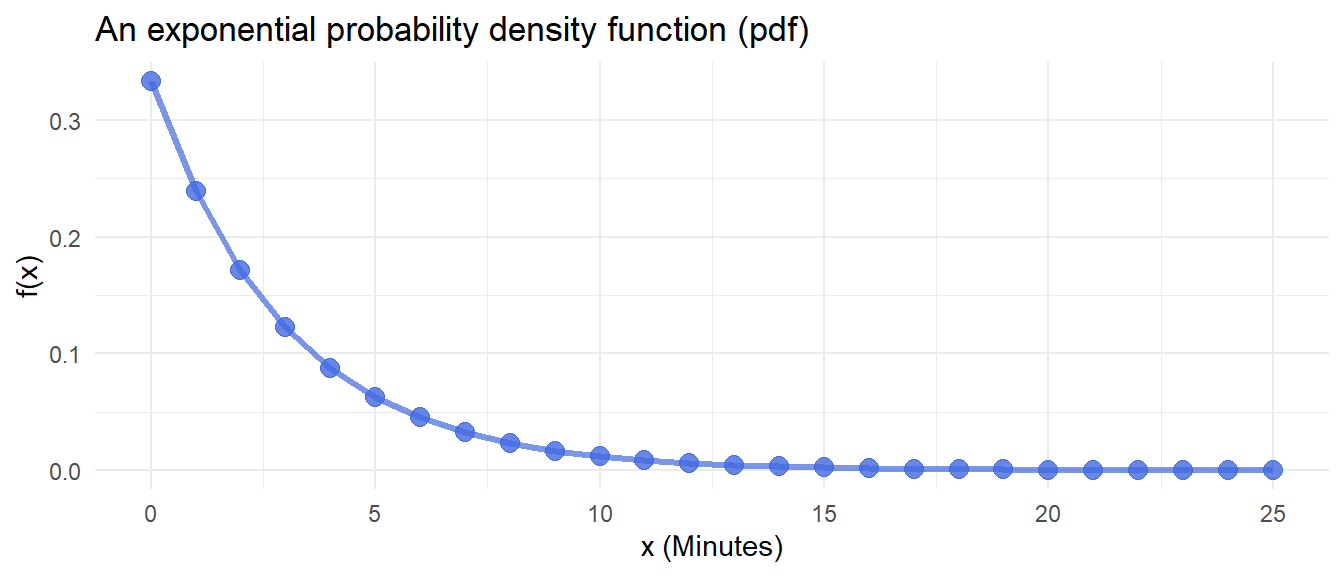
We set the equation up in `R` and plot it so that we can understand what
it represents.
```{r}
P_x <- function(x, beta=3) {
  case_when(x < 0 ~ 0,
            x >= 0 ~ (1/beta) * exp(-x/beta)
            )
}
```
```{r}
#| code-fold: true
#| fig-height: 3
#| warning: false
data <- data.frame(x = x_vec, y = P_x(x_vec))
ggplot(data, aes(x = x, y = y)) +
  geom_point(color = "royalblue", size=3.1, alpha=.8) +
  geom_line(color = "royalblue", size=1.2, alpha=.7) +
  labs(x = "x (Minutes)", y = "f(x)", title = "An exponential probability density function (pdf)") +
  theme_minimal()
```
At each $x$, this function outputs the probability that it takes $x$
minutes placing an order in the drive-thru. For example, the probability
that it takes exactly six minutes to place an order is as follows:
```{r}
P_x(6)
```
That's what a pdf gives us and that's cool. However, our question asks
for the probability that it takes *less than or equal to six minutes to order*. That
involves adding up all of the probabilities for times $[0,6]$ over this
continuous function -- sounds like an integral. Indeed, we'll need to
integrate over the following region:
```{r}
#| code-fold: true
plot_ly(
  x = x_vec,
  y = P_x(x_vec),
  type = "scatter",
  mode="line",
  name = "P(x)") %>% add_trace(
    x = 0:6,
    y = P_x(0:6, 3),
    type = "scatter",
    mode="none",
    fill = "tozeroy",
    name = "P(x) <= 6"
) %>%
  layout(plot_bgcolor = "#e5ecf6", shapes = list(vline(6))
         )
```
We can formally define that integral as follows:
$$
\begin{align*}
P(X \leq 6) &= \int_0 ^6 f(x)dx \\
&= \int_0 ^6 \frac{1}{\beta} e^{-\frac{x}{\beta}}dx
\end{align*}
$$
Now that we've defined the problem, we'll solve it by-hand, then using symbolic computation software.
### Solving by hand
After setting the problem up, we can solve it step-by-step using $u$ substitution to compute the integral:
$$
\begin{align*}
P(X \leq 6) &= \int_0 ^6 \frac{1}{\beta} e^{-\frac{x}{\beta}}dx \\
\text{Substitute}\, u &= -\frac{x}{\beta} \\
\text{And substitute}\, dx \rightarrow \, \frac{du}{dx} &= -\frac{1}{\beta} \rightarrow dx = -\beta du \\
P(X \leq 6) &= \int_0 ^6 \frac{1}{\beta} e^u (-\beta du) \\
&= -1\int_0 ^6 e^u du \\
&= - e^u \Big|_0^6 \\
P(X \leq 6) &= - e^{-\frac{x}{\beta}} \Big|_0^6 \\
\end{align*}
$$
The last line gives us the following algebra:
$- e^{-\frac{x}{\beta}} \Big|_0^6 = - e^{-\frac{6}{3}} - (- e^{-\frac{0}{3}}) = 1 - e^{-\frac{6}{3}}$
Leading us to our answer:
```{r}
(-exp(-6/3)) + 1
```
Which is the probability that it takes six minutes or less to order in
this drive-thru.
### Solving with `sympy`
Now we'll overview a more practically useful way of solving the integral using python's `sympy` library. To switch to python, I'll first load the `reticulate` library in R and specify that I want to use my conda install of python, which comes pre-loaded with `sympy`.
```{r}
#| warning: false
library(reticulate)
use_condaenv('base')
```
Now I'll switch to python code and set up some preliminaries -- I define a custom render function so that I can output the `sympy` equations I create in LaTeX:
```{python filename="python"}
import sympy as sp
from IPython.display import Markdown
render = lambda x: Markdown(sp.latex(x, mode='equation'))
```
Now I'll define the variables, the constant $e$,^[This is not strictly necessary -- I do it purely so that I can reference `e` in my code and match the problem notation] and @eq-uni-pdf in `sympy`. `sympy` will automatically apply some simplification to the expression, so don't worry if it doesn't look exactly like @eq-uni-pdf.
```{python filename="python"}
# Define the variables
x, beta = sp.symbols('x beta')
# Define the constant, e
e = sp.exp(1)
# Define the equation
pdf = (1/beta) * e**(-x/beta)
# Render the equation
render(pdf)
```
In our specific problem, we know that the average time it takes to place an order is 3, so we'll substitute in $\beta=3$.
```{python filename="python"}
f_x = pdf.subs({beta: 3})
render(f_x)
```
Integration using `sympy` is trivially easy -- to get the indefinite integral, we can just call `.integrate()` and supply the variable of integration.
```{python filename="python"}
render(f_x.integrate(x))
```
The problem requires the definite integrate, which is just as straightforward -- we supply the variable to integrate over, and the upper and lower limits of integration.
```{python filename="python"}
render(f_x.integrate( (x, 0, 6) ))
```
We'll retrieve the decimal output by running `.evalf()` on the integral.
```{python filename="python"}
f_x.integrate( (x, 0, 6) ).evalf()
```
Much less painful than $u$-substitution!
## Cumulative Probability
When we derived the indefinite integral,
$\int \frac{1}{\beta} e^{-\frac{x}{\beta}}dx = - e^{-\frac{x}{\beta}}$,
in the process of solving our definite integral problem, we actually
derived another useful function – the cumulative distribution function (cdf).
The cumulative distribution function describes the probability that $x$ is some number, say $a$, or less, and it is generally the integral of the
probability density function [@noauthor_cumulative_2024]. In the case of the exponential function,
it is as follows:
$$
F(a) = P(x \leq a) = \int_0^a P(x)dx =- e^{-\frac{x}{\beta}} \Big|_0^a
$$
Or, in code:
```{r}
cdf_x <- function(x, beta=3){
  -1 * exp(-x/beta)
}
```
We'll confirm that $F(6) = e^{-\frac{x}{\beta}} \Big|_0^6$
```{r}
1 + cdf_x(6)
```
Here are the pdf and cdf functions plotted together for the exponential
distribution with an average of 3 ($\beta=3$). At each point on the
orange line (the pdf), you can hover over and find out the probability
that the drive-thru takes exactly $x$ minutes, whereas on the blue line
(the cdf), you'll find the probability that the drive-thru takes less
than or equal to $x$ minutes.
```{r}
#| code-fold: true
plot_ly(
  x = x_vec,
  y = 1 + cdf_x(x_vec),
  type = "scatter",
  mode="lines+markers",
  name = "CDF: F(a)") %>%
  add_trace(
    x = x_vec,
    y = P_x(x_vec),
    type = "scatter",
    mode="lines+markers",
    name = "PDF: P(x)"
)
```
## Modeling multiple waiting times
> At Sydney’s Restaurant, customers must wait an average of 15 minutes
> for a table. From the time they are seated until they have finished
> their meal requires an additional 40 minutes, on average. What is the
> probability that a customer spends less than an hour and a half at the
> diner, assuming that waiting for a table and completing the meal are
> independent events?
>
> -- [@strang_calculus_2016-1, chapter 5.2]
Since we are given two random variables and asked to find the
probability of an event where something specific happens to each one, we
can conceive of this problem using a joint density function. We are given
that these two waiting times are independent (not correlated), so we can
model joint density as follows:
> The variables $X$ and $Y$ are said to be independent random variables
> if their joint density function is the product of their individual
> density functions: $$
> f(x, y) = f_1(x)f_2(y)
> $$
>
> -- [@strang_calculus_2016-1, chapter 5.2]
The two functions given in the problem are:
1. an exponential density function with mean 15 (waiting for the table)
$$
f_1(x) = \begin{cases}
\frac{1}{15} e^{-\frac{x}{15}} \quad &x \geq 0 \\
0 \quad &x < 0
\end{cases}
$$
2. an exponential density function with mean 40 (eating at the table)
$$
f_2(y) = \begin{cases}
\frac{1}{40} e^{-\frac{y}{40}} \quad &y \geq 0 \\
0 \quad &y < 0
\end{cases}
$$
This gives us the joint density function:
$$
\begin{align*}
f(x, y) &= f_1(x)f_2(y) \\
&= \left[\begin{cases}
\frac{1}{40} e^{-\frac{x}{40}} \quad &x \geq 0 \\
0 \quad &x < 0
\end{cases} \right] \times \left[ \begin{cases}
\frac{1}{15} e^{-\frac{y}{15}} \quad &y \geq 0 \\
0 \quad &y < 0
\end{cases} \right] \\
&=
\begin{cases}
\frac{1}{600} e^{-\frac{x}{40}}e^{-\frac{y}{15}} \quad &x,y \geq 0 \\
0 \quad &x < 0 \,\text{or}\, y < 0
\end{cases}
\end{align*}
$${#eq-syd}
We can set that up in code as well
```{r}
pdf_function <- function(x, y) {
  table_wait <- P_x(x, 15)
  eating_time <- P_x(y, 40)
  total_time <- table_wait * eating_time
  return(total_time)
}
```
This function allows us to find the probability of our table wait +
eating time being a specific amount of minutes. For example, what's the
probability that it takes us 15 minutes to secure a table and 40 minutes
to eat?
```{r}
pdf_function(15, 40)
```
This is a really small number, which makes some level of intuitive sense
-- it seems remote that the whole restaurant experience will take
exactly 55 minutes, no more no less.
Now, returning to the question -- we want to find the probability that
the whole restaurant experience (waiting for a table and eating) takes
an hour and a half (90 minutes) or less. Again, we'll need to add up all of the probabilities from 0 to 90 minutes, implying that we will solve this with an integral. However, we are in a multivariate setting, so this will require multiple integration.
To set up the problem, we'll plot the joint density function, the $xy$ plane, and this 90 minute constraint.
```{python}
#| output: false
#| echo: false
import numpy as np
import matplotlib.pyplot as plt
from mpl_toolkits.mplot3d import Axes3D
# Define the PDF function
def pdf_function(x, y):
# Replace this with the actual PDF function
return np.exp(-0.01 * (x**2 + y**2))
# Define range for x and y
x_range = np.linspace(0, 25, 100)
y_range = np.linspace(0, 25, 100)
x_grid, y_grid = np.meshgrid(x_range, y_range)
# Calculate z values for the surface plot
z_values = pdf_function(x_grid, y_grid)
z_plane = np.zeros_like(z_values)
# Create the plot
fig = plt.figure(figsize=(3, 3))
ax = fig.add_subplot(111, projection='3d')
# Plot the surface
surf = ax.plot_surface(x_grid, y_grid, z_plane, color='lightgrey', alpha=0.5)
surf = ax.plot_surface(x_grid, y_grid, z_values, cmap='coolwarm', alpha=.8)
# Zoom in on the plot by setting axis limits
ax.set_xlim(1, 10)
ax.set_ylim(1, 10)
ax.set_zlim(.1, .7)
ax.view_init(elev=3, azim=-55)
ax.set_axis_off()
fig.tight_layout()
fig.savefig("thumbnail.png", dpi=300)
plt.show()
```
```{r}
#| warning: false
#| code-fold: true
scene <- list(
  camera = list(eye = list(
    x = 2, y = 1.1, z = 1.2
  )),
  xaxis = list(title = "X"),
  yaxis = list(title = "Y"),
  zaxis = list(title = "P(X,Y)")
)
# Define range for x and y
x_range <- seq(0, 50, length.out = 100)
y_range <- seq(0, 50, length.out = 100)
xy_grid <- expand.grid(x = x_range, y = y_range)

z_values <- pdf_function(xy_grid$x, xy_grid$y)
z_plane <- rep(0, nrow(xy_grid))

# x y constraint
x_range_constraint <- seq(40, 50, length.out = 100)
y_constraint <- 90 - x_range_constraint
xy_constraint_grid <- expand.grid(x = x_range_constraint, y = y_constraint)
z_constraint <- rep(0, nrow(xy_grid))


# Reshape z values to create a matrix for plotting
z_matrix <- matrix(z_values, nrow = length(x_range), ncol = length(y_range))
z_constraint_matrix <- matrix(z_constraint, nrow = length(x_range), ncol = length(y_constraint))
z_plane_matrix <- matrix(z_plane, nrow = length(x_range), ncol = length(y_range))


# Create 3D plot using plot_ly
plot_ly(x = x_range, y = y_range, z = z_plane_matrix, type = "surface") %>% hide_colorbar() %>%
  add_trace(
    x = x_range,
    y = y_range,
    z = z_matrix,
    type = "surface",
    colorscale = "Cividis",
    colorbar = list(title = "P(X,Y)")
  ) %>%
  add_trace(
    x = x_range_constraint,
    y = y_constraint,
    z = 0,
    type = "scatter3d",
    name = "X + Y <= 90",
    mode="lines+markers"
  ) %>% layout(scene = scene)
```
Let's first define a region of integration, $D$. We are given $x+y \leq 90$, and given that we are talking about minutes, which are bounded $[0, \infty)$, we can make that $0 \leq x+y \leq 90$. With some algebraic manipulation, we can define the region as:
$$
D = \{(x,y) \,|\, 0 \leq x \leq90, 0 \leq y \leq 90-x \}
$$
Setting that up as a definite integral, we get the following:
$$
P(X+Y \leq 90) = P( (X,Y) \in D) = \iint_D f(x,y) dA
$$
Given that there is no density for this function when $x$ or $y$ is less than zero, we can ignore the piece wise structure of the joint pdf and set up the integral using only the portion that defines the function on the domain $x \in [0, \infty)$. This gives us:
$$
\begin{align*}
&= \int_0^{90} \int_0^{90-x} \frac{1}{600} e^{-\frac{x}{40}}e^{-\frac{y}{15}} dydx \\
&= \frac{1}{600} \int_0^{90} \int_0^{90-x} e^{-\frac{x}{40}-\frac{y}{15}} dydx
\end{align*}
$$
### Solving by hand
Computing this integral is difficult, but we'll walk through it. We will again use $u$ substitution.
$$
\begin{align*}
u &= -\frac{x}{40}-\frac{y}{15} \\
\frac{du}{dy} &= -\frac{1}{15} \rightarrow dy=-15du\\
\end{align*}
$$
We can plug that in to finish the first integral:
$$
\begin{align*}
&= \frac{1}{600}\int_0^{90} \int_0^{90-x} e^{u} (-15)dudx \\
&= \frac{-15}{600}\int_0^{90} \int_0^{90-x} e^{u} dudx \\
&= \frac{-15}{600}\int_0^{90} e^{u} \Big|_0^{90-x} dx \\
&= \frac{-15}{600}\int_0^{90} e^{-\frac{x}{40}-\frac{y}{15}} \Big|_0^{90-x} dx \\
&= \frac{-15}{600}\int_0^{90} e^{-\frac{x}{40}-\frac{90-x}{15}} - e^{-\frac{x}{40}-\frac{0}{15}} dx \\
&= \frac{-15}{600}\int_0^{90} e^{-\frac{3x}{120}-\frac{8(90-x)}{120}} - e^{-\frac{x}{40}}dx \\
&= \frac{-15}{600}\int_0^{90} e^{\frac{-3x-720+8x}{120}} - e^{-\frac{x}{40}}dx \\
&= \frac{-15}{600}\int_0^{90} e^{\frac{5x-720}{120}} - e^{-\frac{x}{40}}dx \\
&= \frac{-15}{600}\int_0^{90} e^{\frac{x}{24}-6} - e^{-\frac{x}{40}}dx
\end{align*}
$$
That was pretty difficult! Now we can continue on to the second integral and split it into two:
$$
\begin{align*}
&= \frac{-15}{600} \left[ \int_0^{90} e^{\frac{x}{24}-6}dx - \int_0^{90} e^{-\frac{x}{40}}dx \right]
\end{align*}
$$
We'll solve these integrals with $u$ and $v$ substitution, with our terms defined as follows:
$$
\begin{align*}
u &= \frac{x}{24}-6 \\
\frac{du}{dx} &= \frac{1}{24} \rightarrow dx=24du\\
v &= -\frac{x}{40} \\
\frac{dv}{dx} &= -\frac{1}{40} \rightarrow dx=-40dv\\
\end{align*}
$$
When we plug these terms back in, we can finally compute the definite integral.
$$
\begin{align*}
&= \frac{-15}{600} \left[ 24 \int_0^{90} e^{u}du + 40\int_0^{90} e^v dv \right] \\
&= \frac{-15}{600} \left[ 24 e^{u}\Big|_0^{90} + 40 e^v \Big|_0^{90} \right] \\
&= \frac{-15}{600} \left[ 24 e^{\frac{x}{24}-6}\Big|_0^{90} + 40 e^{-\frac{x}{40}}\Big|_0^{90} \right] \\
&= \frac{-15}{600} \left[24(e^{\frac{90}{24}-6} - e^{\frac{0}{24}-6}) + 40(e^{-\frac{90}{40}}-e^{-\frac{0}{40}}) \right] \\
&= \frac{-15}{600} \left[24(e^{-2.25} - e^{-6}) + 40(e^{-2.25}-1) \right] \\
&= \frac{-15}{600} \left[ -33.3139396802807 \right] \\
&= 0.832848492007017
\end{align*}
$$
Thus, the probability that the total experience is 90 minutes or less is about 83%.
### Solving with `sympy`
Computing that double integral by hand provides us with a lot of opportunities to make a small error and break the whole computation. In practice, we can solve problems like this in a much faster and less error-prone manner using symbolic computation software. We'll again switch to python and use `sympy`.
Returning to the problem,
$$
P(X+Y \leq 90) = \frac{1}{600} \int_0^{90} \int_0^{90-x} e^{-\frac{x}{40}-\frac{y}{15}} dydx
$$
We'll first define the function that we are integrating over.
```{python filename="python"}
# Define the variables
x, y, = sp.symbols("x y")
# Define the function
f_x_y = e ** (-x/40 - y/15)
render(f_x_y)
```
Now, we'll compute the entire double integral in one line. Note that we chain the `.integrate()` method, each time over a different variable, to perform the multiple integration.
```{python filename="python"}
(1/600) * (
  f_x_y
  .integrate( (y, 0, 90-x) )
  .integrate( (x, 0, 90) )
  .evalf()
  )
```
We confirm that this is the same answer we arrived at by hand.
## Deriving a generalizable approach
Let's look at another problem, but now, instead of solving just one specific problem, we'll derive an equation that can easily solve any question structured like this so that don't have to do so many integrals...
>[...] At a drive-thru restaurant, customers spend, on average, 3 minutes placing their orders and an additional 5 minutes paying for and picking up their meals. Assume that placing the order and paying for/picking up the meal are two independent events $X$ and $Y$. If the waiting times are modeled by the exponential probability densities. Find $P[X+Y \leq 6]$ and interpret the result.
>
> -- [@strang_calculus_2016-1, chapter 5.2] - Question 119
We'll again set up the joint density function:
$$
\begin{align*}
f(x, y) &= f_1(x)f_2(y) \\
&= \left[\begin{cases}
\frac{1}{3} e^{-\frac{x}{3}} \quad &x \geq 0 \\
0 \quad &x < 0
\end{cases} \right] \times \left[ \begin{cases}
\frac{1}{5} e^{-\frac{y}{5}} \quad &y \geq 0 \\
0 \quad &y < 0
\end{cases} \right] \\
&=
\begin{cases}
\frac{1}{15} e^{-\frac{x}{3}}e^{-\frac{y}{5}} \quad &x,y \geq 0 \\
0 \quad &x < 0 \,\text{or}\, y < 0
\end{cases}
\end{align*}
$$
and the region of integration appropriate for answering the question:
$$
D = \{(x,y) \,|\, 0 \leq x \leq6, 0 \leq y \leq 6-x \}
$$
This leaves us with the integral:
$$
\begin{align*}
\frac{1}{15} \int_0^{6} \int_0^{6-x} e^{-\frac{x}{3}-\frac{y}{5}} dydx
\end{align*}
$$
However, rather than solve this specifically, lets take the opportunity to derive a more general solution that can give us the target probability for **any question phrased like this.**
We'll replace all the specific values:
- 3, which is the average amount of minutes in the drive-thru, with $\beta_1$,
- 5, which is the average amount of minutes spent ordering, with $\beta_2$, and
- 6, which is the maximum number of minutes for the whole experience, with $c$.
That gives us:
$$
\begin{align*}
&= \frac{1}{\beta_1\beta_2} \int_0^{c} \int_0^{c-x} e^{-\frac{x}{\beta_1}-\frac{y}{\beta_2}} dydx
\end{align*}
$$
### Solving by hand
Let's walk through one more painful double integral by-hand. We'll start with $u$ substitution:
$$
\begin{align*}
u &= -\frac{x}{\beta_1}-\frac{y}{\beta_2} \\
\frac{du}{dy} &= -\frac{1}{\beta_2} \rightarrow dy=-\beta_2du\\
\end{align*}
$$
And plug those in to solve the first definite integral:
$$
\begin{align*}
&= \frac{-1}{\beta_1} \int_0^{c} \int_0^{c-x} e^{u} dudx \\
&= \frac{-1}{\beta_1}\int_0^{c} e^{-\frac{x}{\beta_1}-\frac{y}{\beta_2}} \Big|_0^{c-x} dx \\
&= \frac{-1}{\beta_1}\int_0^{c} e^{-\frac{x}{\beta_1}-\frac{c-x}{\beta_2}} - e^{-\frac{x}{\beta_1}-\frac{0}{\beta_2}} dx \\
&= \frac{-1}{\beta_1}\int_0^{c} e^{-\frac{\beta_2x}{\beta_1\beta_2}-\frac{\beta_1(c-x)}{\beta_1\beta_2}} - e^{-\frac{x}{\beta_1}}dx \\
&= \frac{-1}{\beta_1}\int_0^{c} e^{\frac{-\beta_2x - \beta_1c+\beta_1x}{\beta_1\beta_2}} - e^{-\frac{x}{\beta_1}}dx \\
&= \frac{-1}{\beta_1} \left[ \int_0^{c} e^{\frac{(\beta_1-\beta_2)x - \beta_1c}{\beta_1\beta_2}}dx - \int_0^{c} e^{-\frac{x}{\beta_1}}dx \right] \\
\end{align*}
$$
Now we'll use $u$ and $v$ substitution to solve the last definite integral:
$$
\begin{align*}
u &= \frac{(\beta_1-\beta_2)x - \beta_1c}{\beta_1\beta_2} \\
\frac{du}{dx} &= \frac{(\beta_1-\beta_2)}{\beta_1\beta_2} \rightarrow dx=\frac{\beta_1\beta_2}{(\beta_1-\beta_2)}du\\
v &= -\frac{x}{\beta_1} \\
\frac{dv}{dx} &= -\frac{1}{\beta_1} \rightarrow dx=-\beta_1dv\\
\end{align*}
$$
Plugging those in, we arrive at a general function of $\beta_1$, $\beta_2$, and $c$.
$$
\begin{align*}
&= \frac{-1}{\beta_1} \left[ \int_0^{c} e^{u}\frac{\beta_1\beta_2}{(\beta_1-\beta_2)}du - \int_0^{c} e^{v}(-\beta_1dv) \right] \\
&= \frac{-1}{\beta_1} \left[ \frac{\beta_1\beta_2}{(\beta_1-\beta_2)}\int_0^{c} e^{u}du - (-\beta_1)\int_0^{c} e^{v}dv \right] \\
&= \frac{-1}{\beta_1} \left[ \frac{\beta_1\beta_2}{(\beta_1-\beta_2)} (e^{\frac{(\beta_1-\beta_2)x - \beta_1c}{\beta_1\beta_2}}\Big|_0^{c}) + \beta_1 (e^{-\frac{x}{\beta_1}}\Big|_0^{c}) \right] \\
&=\left[ \frac{-\beta_2}{(\beta_1-\beta_2)} (e^{\frac{(\beta_1-\beta_2)c - \beta_1c}{\beta_1\beta_2}} - e^{\frac{-\beta_1c}{\beta_1\beta_2}}) - (e^{-\frac{c}{\beta_1}} - e^{-\frac{0}{\beta_1}}) \right] \\
&= \frac{-\beta_2}{(\beta_1-\beta_2)} \left[e^{\frac{(\beta_1-\beta_2)c - \beta_1c}{\beta_1\beta_2}} - e^{\frac{-\beta_1c}{\beta_1\beta_2}}\right] - e^{-\frac{c}{\beta_1}} + 1 \\
f(\beta_1, \beta_2, c)&= \frac{-\beta_2}{(\beta_1-\beta_2)} \left[e^{\frac{-c}{\beta_1}} - e^{\frac{-c}{\beta_2}}\right] - e^{-\frac{c}{\beta_1}} + 1 \\
\end{align*}
$$
Now we'll code that equation up in `R` or the calculator of your choice.
```{r}
cdf_wait <- function(beta1, beta2, c) {
  (-beta2/(beta1-beta2)) *
  (exp((-c)/beta1) - exp((-c)/beta2)) -
  exp((-c)/beta1) + 1
}
```
Going back to our question -- let's see what's the probability that the drive-thru experience takes 6 minutes or less if waiting to order takes 3 minutes on average and ordering takes 5 minutes on average. We can very easily calculate it with the flexible function $f(\beta_1, \beta_2, c)$ that we just derived:
```{r}
cdf_wait(3, 5, 6)
```
There's a ~45% chance that a customer will spend 6 minutes or less in the drive-thru. We can also use our function, $f(\beta_1, \beta_2, c)$, to easily compute and visualize the probability for any total drive-thru time given these two average times.
```{r}
#| code-fold: true
plot_ly(
  x = x_vec,
  y = cdf_wait(3, 5, x_vec),
  type = "scatter",
  mode="lines+markers",
  name = "CDF: F(a)")
```
And, going back to the first multiple integration question about Sydney's restaurant @eq-syd, we can now answer that with the same function.
```{r}
cdf_wait(15, 40, 90)
```
We again can find the cumulative probability for any waiting time given the average time to get a table (15) and eat (40).
```{r}
#| code-fold: true
plot_ly(
  x = seq(0, 150),
  y = cdf_wait(15, 40, seq(0, 150)),
  type = "scatter",
  mode="lines+markers",
  name = "CDF: F(a)")
```
### Solving with `sympy`
For the sake of completeness, we'll derive that same generizable equation using `sympy`. Returning to the problem,
$$
\begin{align*}
P(X + Y \leq x) &= \frac{1}{\beta_1\beta_2} \int_0^{c} \int_0^{c-x} e^{-\frac{x}{\beta_1}-\frac{y}{\beta_2}} dydx
\end{align*}
$$
we'll define the constants and function in `sympy`.
```{python filename="python"}
x, y = sp.symbols('x y')
beta1, beta2, c = sp.symbols('beta1 beta2 c')
f_x_y_general = e**(-x/beta1 - y/beta2)
render(f_x_y_general)
```
We compute the double integral, and define our generalizable function as `f_b1_b2_c`.
```{python filename="python"}
f_b1_b2_c = ( 1/(beta1 * beta2) ) * (
  f_x_y_general
  .integrate( (y, 0, c - x) )
  .integrate( (x, 0, c) )
)
render(f_b1_b2_c.simplify())
```
Note that for more complex equations like this, `sympy`'s simplified output might not look like what you'd reach by hand. We can be more confident that this is indeed the same $f(\beta_1, \beta_2, c)$ as the one we computed by hand above by testing it with a few problems and confirming the expected output.
Returning to the drive-thru experience, where waiting to order takes 3 minutes on average and ordering takes 5, we can compute the probability that the whole experience takes 6 minutes or less as follows:
```{python filename="python"}
f_b1_b2_c.subs({beta1: 3, beta2: 5, c:6}).evalf()
```
This is the same as what we get using the by-hand function.
```{r}
cdf_wait(3, 5, 6)
```
In the case of the first problem, with a restaurant where ordering takes 40 minutes on average and eating takes 15, we can compute the probability that the whole experience takes 90 minutes or less just as easily:
```{python filename="python"}
f_b1_b2_c.subs({beta1: 40, beta2: 15, c:90}).evalf()
```
Again, let's check this with the by-hand version.
```{r}
cdf_wait(15, 40, 90)
```
Great!